Most sizable neural networks today rely on backpropogation to make the training process more efficient. While backpropogation is pretty ubiquitous in libraries such as torch.autograd, I was curious how difficult it would be to implement it myself without using existing helpers. Turns out: not that difficult, and can be done with ~200 lines of Python!
In this two-part blog post, we’ll derive backpropogation from scratch, implement it, and use it to train a simple neural network. Crucially, for learning purposes, we won’t be using libraries like Torch or autodiff; rather, we will use only vanilla Python and numpy for matrix operations. I’ve also tried to strike a balance between simplicity and depth, so that anyone with a passing understanding of matrices and derivatives should be able to follow along.
Background
A neural network consists of a number of “neurons” connected via layers that work together to produce some output. A simple three-layer, fully-connected neural network can be seen below. 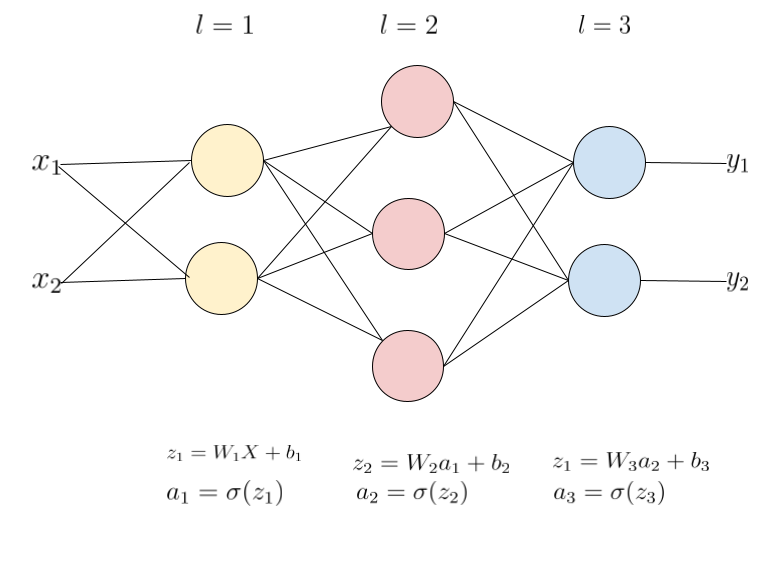
3-layer neural network
In this example, we have two inputs, \(x_1\) and \(x_2\), that go through three layers before producing the final output, consisting of \(y_1\) and \(y_2\). Each layer \(l\) of neurons:
- takes some input from the previous layer \(l-1\)
- transforms it by multiplying the input by a weight matrix \(W_l\) and adding a bias term \(b_l\)
- applies an activation function \(\sigma()\)
- then finally, passes the output to the next layer \(l+1\)
This type of neural network, where information flows in only one direction - from the input layer to the output layer - is called a feedforward neural network.
The “training process”, then, consists of finding the optimal weights and biases in the network such that some cost function is minimized. The cost function can be seen as how poorly the network performs, so lower is better. The hope is that given enough training data and iterations, we can reduce the cost function to a minimum, which by extension means the network will do a pretty good job of predicting an output.
Below is some notation to formalize this idea.
- \(L\): number of layers in the network, including hidden layers and the output layer. The above example has \(L = 3\).
- \(X\): input set, consisting of \(x_1, x_2, ... , x_n\)
- \(W_l\): weight matrix of layer \(l\) where \(w^l_{ij}\) is the weight of the connection between the \(i\)th neuron of layer \(l\) and the \(j\)th neuron of layer \(l-1\). This is a matrix with size \(n \times m\), where \(n\) is the number of neurons in the current layer and \(m\) is the number of inputs to the current layer.
- \(z_l\): the weighted sum of all inputs into layer \(l\). This is a vector with number of rows = number of neurons in layer \(l\).
- \(a_l\): the activation of layer \(l\), equal to \(\sigma(z_l)\). This is a vector with number of rows = number of neurons in layer \(l\).
- \(C()\): cost function. For a single training sample, we’ll use \(\begin{align}\frac{1}{2}(y_i - \hat{y_i})^2\end{align}\) where \(y_i\) is the training sample and \(\hat{y_i}\) is the predicted value. For multiple training samples \(n\), we’ll use the mean squared error, defined as \(\begin{align}\frac{1}{2n}\sum_{i=1}^n(y_i - \hat{y_i})^2\end{align}\).
- \(\sigma()\): activation function. In this example we’ll use the sigmoid function, defined as \(\begin{align}\sigma(x) = \frac{1}{1 + e^{-x}}\end{align}\).
But how do we adjust the weights and biases? A common method of doing this is via gradient descent. Since we want to minimize some cost function, gradient descent essentally finds the gradient of the function at some point, then moves the weights and biases in the opposite direction of the gradient. Keep in mind that gradient descent only finds a local minimum and not a global minimum. 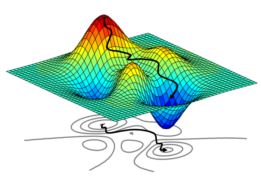
Finding local minima via gradient descent
How to efficiently find the gradient of the cost function with respect to each of the input weights and biases is where backpropogation comes into play.
Derivation
For each layer \(l\), we want to find the gradient of the cost function with respect to its weights and biases, or \(\begin{align}\frac{\partial C}{\partial W_l}\end{align}\) and \(\begin{align}\frac{\partial C}{\partial b_l}\end{align}\) respectively. The key intuition is that the derivatives of each layer can be calculated using the derivatives of the next. So by iterating backwards starting from the output layer, we can cache calculated values and reuse them on the next iteration.
The key ingredient of backpropogation is the chain rule of calculus. That is, if \(z = f(y)\) and \(y = f(x)\), then: \(\begin{align} \frac{\partial z}{\partial x} &= \frac{\partial z}{\partial y} \frac{\partial y}{\partial x}.\\ \end{align}\)
Weight updates for output layer
Recall the relationship between \(W_l\), \(z_l\), \(a_l\), and \(C\). \(W_l\) is left-multiplied with the output activation from the previous layer \(a_{l-1}\) to form \(z_l\). \(z_l\) is passed into our activation function \(\sigma\) to form \(a_l\). This process is repeated until the final activation \(a_L\) is passed to the cost function \(C\).
\[\begin{align} z_l &= W_la_{l-1}\\ a_l &= \sigma(z_l)\\ C(a_L) &= \frac{1}{2}(a_{L} - y)^2\\ \end{align}\]Deriving \(\begin{align}\frac{\partial C}{\partial W_L}\end{align}\) for output layer is thus: \(\begin{align} \frac{\partial C}{\partial W_L} &= \frac{\partial C}{\partial a_L}\frac{\partial a_L}{\partial z_L}\frac{\partial z_L}{\partial w_L}\\ &= \frac{\partial}{\partial a_{L}}\frac{1}{2}(a_{L} - y)^2 \odot \sigma'(z_L) \frac{\partial z_L}{\partial W_L}\\ \tag{1.1} &= (a_L - y) \odot \sigma'(z_L) \frac{\partial z_L}{\partial W_L}\\ \end{align}\)
where \(\odot\) is the element-wise product, or Hadamard product, as opposed to regular matrix product. The derivative of the sigmoid function \(\sigma'(x)\) is conveniently:
\[\begin{align} \sigma'(x) &= x(1 - x)\\ \end{align}\]Here we can simplify our notation by defining a new value, \(\delta_l\), as the partial derivative of the cost in terms of our weighted input \(z_l\):
\[\begin{align} \delta_l = \frac{\partial C}{\partial z_l} \end{align}\]So for our output layer \(L\):
\[\begin{align} \tag{2.1} \delta_L = \frac{\partial C}{\partial z_L} = (a_L - y) \odot \sigma'(z_L)\\ \end{align}\]We can now substitute \(\delta_L\) into Equation 1.1:
\[\begin{align} \frac{\partial C}{\partial W_l} &= \delta_L\frac{\partial z_L}{\partial W_L}\\ &= \delta_L\frac{\partial (W_La_{L-1})}{\partial W_L}\\ \tag{1.2} &= \delta_L(a_{L-1})^T \end{align}\]Observe that \(\delta_L\) and \(a_{L-1}\) are vectors of equal dimensions, so we take the transpose of the latter to get an inner product.
Intuitively, \(\delta_l\) represents the “error,” or how sensitive the output of the cost function is in terms of the current layer’s weighted input \(z_l\). If this value is large, that means the cost can be significantly reduced given a small change in the weighted input, so the weighted input \(z_l\) is pretty far off from the desired value. Conversely, a small \(\delta\) means we can’t reduce the cost much more, and thus it is close to the desired value.
Weight updates for hidden layers
For the hidden layers, the relationship between the weights and the final cost is a bit more implicit. But essentially it is a repeated application of the chain rule from some \(W_l\), through the network, and ending at the cost function.
\[\begin{align} \tag{3.1} \frac{\partial C}{\partial W_l} &= \frac{\partial C}{\partial a_L}\frac{\partial a_L}{\partial z_L}\frac{\partial z_L}{\partial W_L}\frac{\partial W_L}{\partial a_{L-1}}\frac{\partial a_{L-1}}{\partial z_{L-1}}\frac{\partial z_{L-1}}{\partial W_{L-1}} ... \frac{\partial a_{l+1}}{\partial z_{l+1}}\frac{\partial z_{l+1}}{\partial W_{l+1}}\frac{\partial W_{l+1}}{\partial a_l}\frac{\partial a_l}{\partial z_l}\frac{\partial z_l}{\partial W_l}\\ \end{align}\]Given our definition of the error term \(\delta_l\) above, we can substitute \(\begin{align}\delta_{l+1} = \frac{\partial C}{\partial z_{l+1}}\end{align}\):
\[\begin{align} \tag{3.2} \frac{\partial C}{\partial W_l} &= \delta_{l+1}\frac{\partial z_{l+1}}{\partial W_{l+1}}\frac{\partial W_{l+1}}{\partial a_l}\frac{\partial a_l}{\partial z_l}\frac{\partial z_l}{\partial W_l}\\ \tag{3.3} &= W_{l+1}^T\delta_{l+1}\frac{\partial a_l}{\partial z_l}\frac{\partial z_l}{\partial W_l}\\ \tag{3.4} &= W_{l+1}^T\delta_{l+1}\frac{\partial \sigma(W_l a_{l-1})}{\partial z_l}\frac{\partial z_l}{\partial W_l}\\ \tag{3.5} &= W_{l+1}^T\delta_{l+1}\odot \sigma'(W_la_{l-1}) \frac{\partial z_l}{\partial W_l}\\ \end{align}\]Alas, we arrive at the key insight of backpropogation. If you compare Equations 3.5 and 3.1, you’ll notice that the entire term \(\begin{align}W_{l+1}^T\delta_{l+1}\odot \sigma'(W_la_{l-1})\end{align}\) is simply \(\begin{align}\frac{\partial C}{\partial z_l}\end{align}\), which is exactly the definition of the error term \(\delta_l\)!
\[\tag{4.1}\begin{align}\delta_l = W_{l+1}^T\delta_{l+1}\odot \sigma'(W_la_{l-1})\end{align}\]What this means is that each error term \(\delta_l\) is defined in terms of its successor \(\delta_{l+1}\). So instead of calculating the entire gradient directly, we can start at the output layer and move backward, saving the error each time so it can be used by the previous layer on the next iteration. In algorithm design, this technique is known as dynamic programming, and it allows us to avoid unnecessary computations.
Finishing up our derivation and substituting in \(\delta_l\):
\[\begin{align} \tag{3.6} \frac{\delta C}{\delta W_l}&= \delta_l \frac{\partial z_l}{\partial W_l}\\ \tag{3.7} &= \delta_l \frac{\partial (W_La_{l-1})}{\partial W_l}\\ \tag{3.8} &= \delta_l (a_{l-1})^T\\ \end{align}\]Last thing to note is that the use of the activations \(a_{l-1}\) means that during the forward pass, these values must be calculated in advance and cached.
Bias updates
Using the above derivation, finding the bias update is much simpler.
\[\begin{align} \frac{\partial C}{\partial b_l} &= \frac{\partial C}{\partial z_l}\frac{\partial z_l}{\partial b_l}\\ &= \delta_l \frac{\partial(W_la_{l-1} + b_l)}{\partial b_l}\\ \tag{5.1} &= \delta_l \end{align}\]Summary of steps
Now that we have all the pieces, we have a algorithm for training a neural network using backpropogation! To summarize:
- For each of \(n\) training samples:
- Forward the input through the network and arrive at a cost, saving the intermediate activations along the way.
- Backpropogate the error term from the last layer to the first layer, i.e. \(\begin{align}\delta_L = (a_L - y)\odot W_La_{L-1}(1 - W_La_{L-1})\end{align}\) for the output layer \(L\) and \(\begin{align}\delta_l = (W_{l+1})^T\delta_{l+1}\odot W_la_{l-1}(1 - W_la_{l-1})\end{align}\) for each hidden layer \(l\).
- To reduce the cost, we can use the errors and activations we saved to find the gradient of the cost function with respect to the weights at each layer, then shift the weights in the opposite direction of the gradient. That is, \(\begin{align} W_l = W_l - \alpha\frac{\partial C}{\partial W_l} \end{align}\) where \(\begin{align}\frac{\partial C}{\partial W_l} = \frac{1}{n}\sum_{i=1}^{n}\delta_{i,l}(a_{i, l-1})^T\end{align}\). Note why we’re including a sum - we have a vector of activations and a vector of errors per training sample, so to calculate a weight update over all training samples we simply take the average.
- Similarly, we update the bias term via \(\begin{align}b_l = b_l - \frac{\alpha}{n} \sum_{i=1}^n\delta_{i,l}\end{align}\).
- Repeat the above steps for a large number of iterations until the cost is sufficiently small.
And that is it! Hopefully that gives us some insight into a key piece of machinery that powers modern deep learning. In the next part of this series, we’ll implement a simple neural network in Python using the backpropogation algorithm we just derived.